Linear Regression between Mental Health and Physical Health
Yuning Wang (yw3438); Aiming Liu (al3998); Qi Lu (ql2370); Yucong Jiang (yj2581); Weiran Zhang (wz2506) 12/02/2019
Motivation
Basic Knowlegde about Mental Health
- Mental health is an important component of overall health.
- Can increases the risk for many types of physical health problems.
- Presence of chronic physical health problems can also increase the risk for mental health problems.
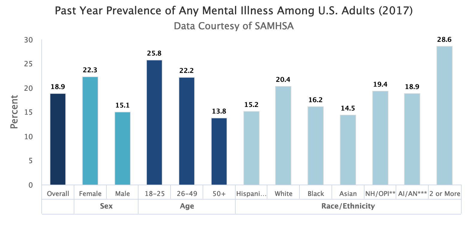
- Over 45 million Americans - almost 20% - are experiencing a mental illness. 57% of adults with a mental illness receive no treatment.
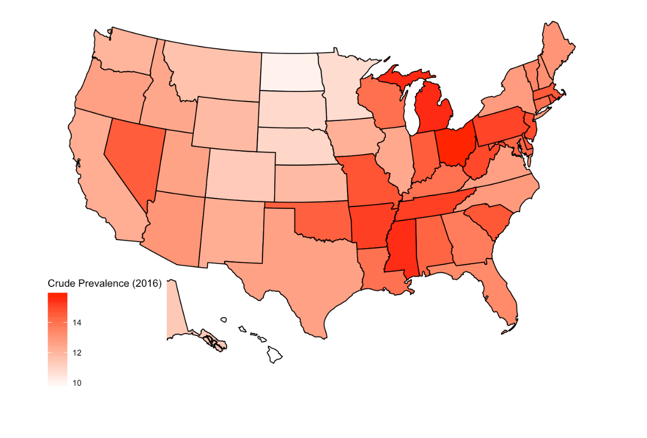
Here’s the map of bad mental health prevalence
The prevalence of mental illness among U.S. adults(2017)
Goals of project
Understanding the risk factors for bad mental health
Visualizing correlation of the risk factors and bad mental health
visualizing the distribution of risk factors and bad mental health prevalence across United States.
Giving suggestions about reducing prevelance of bad mental health
Questions
We tried to figure out the possible causes of bad mental health or mental health illness. We were also interested in visualizing the distribution of risk factors and mental illness prevalence prevalence in the United states, by state and by cities. In addition, we also sought to figure out the correlations between bad mental health and chronic disease and bad living behaviors. As a result, the questions were as followed:
What are the risk factors of bad mental health? What are the correlations between the outcome and the factors? How to visualize them?
What are the distributions of bad mental health and risk factors in different states and cities in the United States? How to visualize them?
Are there any ways for us to reduce the prevalence of bad mental health?
Data
In order to do the analysis, we utilized the 500 Cities: Local Data for Better Health, 2018 release dataset. This dataset includes 2016, 2015 model-based small area estimates for 27 measures of chronic disease related to unhealthy behaviors (5), health outcomes (13), and use of preventive services (9). Data were provided by the Centers for Disease Control and Prevention (CDC), Division of Population Health, Epidemiology and Surveillance Branch. The project was funded by the Robert Wood Johnson Foundation (RWJF) in conjunction with the CDC Foundation. Other datas about U.S. states and territories’ income, U.S. states and territories’ educational attainment and U.S. population race were also used in analyzing the cause of mental health problems.
We downloaded the datasets and filtered the variables that we were interested in and established a new dataset. The risk factors that we are interested in include:
- CANCER: Cancer (excluding skin cancer) among adults aged >= 18 Years
- DIABETES: Diagnosed diabetes among adults aged >=18 Years
- DRINKING: Binge drinking among adults aged >=18 Year
- OBESITY: Obesity among adults aged >=18 Years
- SLEEPING: Sleeping less than 7 hours among adults aged >=18 Years
- INCOME: Median household income in U.S. states and territories
- EDUCATION: Education attainment in U.S. states and territories
- RACE: Population Race in U.S. states and territories
Outcome that we were interested in is:
- MENTAL HEALTH: Mental health not good for >=14 days among adults aged >=18 Years
Analysis
First, we read in the dataset, named it as total_data and filtered the variables that we need.
To make inferences of the relationships between mental health and five variables including obesity, diabetes, drinking, cancer and sleeping which represent the mean prevalence in each cities in the United States in our dataset, we build five linear regression models and plot them. Based on the observations from the five regression models, diabetes, obesity and sleeping have positive association with mental health. drinking and cancer have negative association with mental health.
library(flexdashboard)
library(tidyverse)
library(patchwork)
library(ggridges)
library(viridis)

library(plotly)
# read in the data
mental = read.csv("./data/health data.csv")%>%
janitor::clean_names() %>%
as_tibble() %>%
filter(measure == "mental health" | measure == "obesity" | measure == "diabetes" | measure == "drink" | measure == "cancer" | measure == "sleeping")
mental_data = mental %>%
filter(measure == "mental health")
# read in income, education and ethnicity data
state_stat <- read_csv("data/state_stat.csv")#deal with data
total_data = mental %>%
pivot_wider(names_from = measure, city_name, values_from = data_value) %>%
unnest() %>%
drop_na() %>%
group_by(city_name) %>%
summarize(obesity = mean(obesity), drink = mean(drink), diabetes = mean(diabetes), mental_health = mean(`mental health`), cancer = mean(cancer), sleeping = mean(sleeping))Drink
# Drink
drink_lm = lm(total_data$mental_health ~ total_data$drink, total_data)

drink_plot =
  plot_ly(x = total_data$drink, y = total_data$mental_health,
       type = "scatter",
        mode = "markers",alpha = .5, name = "distribution") %>%
  add_lines(x = total_data$drink, y = fitted(drink_lm), name = "linear model") %>%
  layout(title = 'Binge Drink', colorway = c('#F5B7B1', '#B03A2E'))


drink_plot
From the plots of drinking, we can see a slightly negative relationship. To test if the negative relationship between mental health and drinking is significant or not, we perform a t-test: By using 0.05 significance level, p-value is less than 2e-16, so we can conclude that the negative relationship between mental health and drinking is significant and the regression model is \(Y = -0.30765X + 0.03355\).
Diabetes
# Diabetes
diabetes_lm = lm(total_data$mental_health ~ total_data$diabetes)
diabetes_plot =
  plot_ly(x = total_data$diabetes, y = total_data$mental_health,
       type = "scatter",
        mode = "markers",alpha = .5) %>%
  add_lines(x = total_data$diabetes, y = fitted(diabetes_lm), name = "distribution") %>%
  layout(title = 'Diabetes', colorway = c('#BB8FCE', '#7D3C98'), name = "linear model")


diabetes_plot
For diabetes, we can see from the plot that there is an positive linear relationship and the regression model is \(Y = 0.5985X + 6.7551\). The positive relationship implies people with diabetes will be more likely to have mental health issues.
Cancer
# Cancer
cancer_lm = lm(total_data$mental_health ~ total_data$cancer)

cancer_plot =
  plot_ly(x = total_data$cancer, y = total_data$mental_health,
       type = "scatter",
        mode = "markers",alpha = .5, name = "distribution") %>%
  add_lines(x = total_data$cancer, y = fitted(cancer_lm)) %>%
  layout(title = 'Cancer', colorway = c('#A3E4D7', '#148F77'), name = "linear model")


cancer_plot
From the plot, we can also see a slightly negative association. For the relationship between mental health and cancer, p-value is 0.00149 < 0.05 so we can also conclude that the negative relationship is significant. The regression model is \(Y_i = -0.3275X + 14.7374\)
Obesity
# Obesity
obe_lm = lm(total_data$mental_health ~ total_data$obesity)

obe_plot =
  plot_ly(x = total_data$obesity, y = total_data$mental_health,
       type = "scatter",
        mode = "markers",alpha = .5, name = "distribution") %>%
    add_lines(x = total_data$obesity, y = fitted(obe_lm)) %>%
  layout(title = 'Obesity',colorway = c('#F9E79F', '#D4AC0D'), name = "linear model")


obe_plot
As for the obesity, we can also see a salient positive relationship and the linear regression model is \(Y = 0.26779X + 4.97108\). The positive relationship implies people with obesity will be more likely to have mental health issues.
Sleeping less than 7 hours
#sleeping
sleep_lm = lm(total_data$mental_health ~ total_data$sleeping)

sleep_plot =
  plot_ly(x = total_data$sleeping, y = total_data$mental_health,
       type = "scatter",
        mode = "markers",alpha = .5, name = "distribution") %>%
  add_lines(x = total_data$sleeping, y = fitted(sleep_lm)) %>%
  layout(title = 'Sleeping', colorway = c('#AED6F1', '#2E86C1'), name = "linear model")

sleep_plot
The sleeping variable in our model and plot represents the prevalence of sleeping less than 7 hours, we can see a positive linear relationship between mental health and sleeping which means the cities with more people sleeping less than 7 hours will be more likely to have mental health issues. And the model is \(Y_i = 0.33366X + 1.00842\)
Median Household Income
From this plot we can see that the association between median household income and mental health is significant, i.e. there’s a trend that the higher the household income a state has, the less likely will people in this state have mental illness.
Education Levels
From this plot we can see that there is a significant association between penetration rate of high-school/undergraduate education and the prevalence of bad mental health. Higher penetration rate of high-school/undergraduate education indicates less probability to acquire mental disease. However, there is no significant association between proportion of advanced degress and mental health. We guess that it is because this proportion is too low to affect the statistics of whole population.
Ethnicity
The most concering finding in this plot is that the proportion of black or African-American population is highly and positively related with the prevalence of bad mental health, which corresponds the fact of discrimination. In addition, the proportion of Indian or Asian is negatively related with the prevalence of bad mental health. These facts seem confusing. We guess that it might have been biased by other factors, such as income and education.
Geographic
We used heatmap and plotly to draw the distribution of bad mental health in U.S. states and cities. The distribution of mental health was in similar pattern with that of sleepin less than 7 hours.
Discussion
From the analysis, we gained some ideas about the cause of bad mental health.
In the risk factors that we were interested in, diabetes, obesity and sleeping less than 7 hours have positive relationship with bad mental health. This indicates that chronic diseas are more likely to cause mental health disease. The economic pressure and poor physical conditions caused by chronic diseas might lead to bad mood of the patients and eventually cause a bad mental health and even mental health disease.
Binge drinking, cancer and income are inversely associated with bad mental health. Drinking might be able to release stress, which can enable people to keep a good mood. Individuals who have high income may have less socioeconomic pressure and are more cared about their mental health conditions.
As for level of education,we can see from the results that a high rate of high-school and college education are inversely associated with bad mental health. Thus a higher education level indicates that the person has a better way to adjust the mental condition.
In the aspect of race. It can be discovered that asian and indian have negative relationship with bad mental health while the black has a positive relationship with bad mental health prevalence. This shows that racial discrimination experience that different populations have been through have an effect on the mental health conditions of people.